For a little under a year now, I’ve been using Modo to learn how to create 3D models. I’m doing this partly for fun, and partly to help me think about game engine features from the perspective of an artist. Along with the traditional poly-modeling tools, Modo (like many other 3D tools) also has support for subdivision surfaces. A subdivision surface basically allows you to create a low-poly control mesh for your model, and to add detail, you let the application divide each face in your mesh according to a set of rules.
Here’s an example:
Notice how few polygons there are in the leftmost model. At each increasing level of subdivision to the right, each face gets split into four new faces to add detail. This allows the square hole with sharp edges to become a nice round hole with smooth edges. If you made a mistake (as I frequently do), then it is relatively easy to fix the mistake in the low poly control mesh because there are so few vertices to deal with.
Sounds good, right? Mostly it is, but there is a fairly steep learning curve to subdivision surfaces. One of the main problems is really understanding how your original control mesh relates to the subdivided version. None of the points in the control mesh are guaranteed to remain in the exact same position once the subdivision has occurred, and working out where these points are going to move can sometimes seem like voodoo. In various forums, arguments rage on about edgeloop modeling, E-Poles, N-Poles, keeping only regular vertices, avoiding triangles, n-gons etc. I really wanted to better understand what was going on during subdivision, so I started to dig a little deeper into the details. In the rest of this article, I’m going to share what I’ve learned so far.
A Little Background First
How exactly does a 3D application decide how to subdivide a control mesh? Well, there are a few different subdivision schemes out there, but the most widely used is Catmull-Clark subdivision. Since the original paper by Ed Catmull and Jim Clark, there have been a number of improvements to the original scheme, in particular dealing with crease and boundary edges. This means that although an application might say that it uses Catmull-Clark subdivision, you’ll probably see slightly different results, particularly in regard to edge weights and boundaries.
Rules of Subdivision
The original rules for how to subdivide a control mesh are actually fairly simple. The paper describes the mathematics behind the rules for meshes with quads only, and then goes on to generalize this without proof for meshes with arbitrary polygons. I’m going to go through a very simple example here to show what happens when a mesh gets subdivided. I’m going to be concentrating solely on non-boundary sections of the mesh for simplicity. Also, the example uses a 2D mesh, but again this is only for simplicity, and the principles expand to 3D without change.
There are four basic steps to subdividing a mesh of control-points:
1. Add a new point to each face, called the face-point.
2. Add a new point to each edge, called the edge-point.
3. Move the control-point to another position, called the vertex-point.
4. Connect the new points.
Easy, right? The only question left to answer is, what are the rules for adding and moving these points? Well, like I wrote earlier, this really depends on who implemented it, but I’m going to show the original Catmull-Clark rules using screenshots from Modo. This doesn’t mean that these are the rules that Modo applies, but it should be fairly close.
Here’s the example mesh I’m going to be using:

No prizes for guessing which face we’re going to be looking at. I’ve made it a little bit skewed because that makes things more interesting. If you’re wondering about the double edges around the boundary, I’m going to be writing about those at a later date, so be patient! For now I need them to make the boundary hold shape, but they can be safely ignored for the purposes of this article.
Step One
Firstly, we need to insert a face point, but where? Well this is easy, it just needs to go at the average position of all the control points for the face:

I’ve drawn red dots approximately where each new face-point will go. The big dot is obviously the face-point for the highlighted face. The location for each dot is simply the sum of all the positions of the control-points in that face, divided by the number of control-points.
Step Two
Now we need to add edge-points. Because we’re not dealing with weighted, crease or boundary edges, this is also fairly simple. For each edge, we take the average of the two control points on either side of the edge, and the face-points of the touching faces.
Here’s an example for one edge-point, in blue, where the control points affecting its position are pink, and face-points are red. Note that the edge points don’t necessarily lie on the original edge!
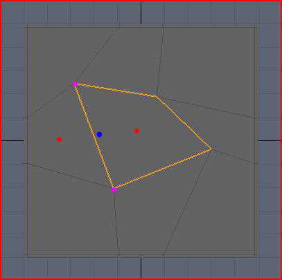
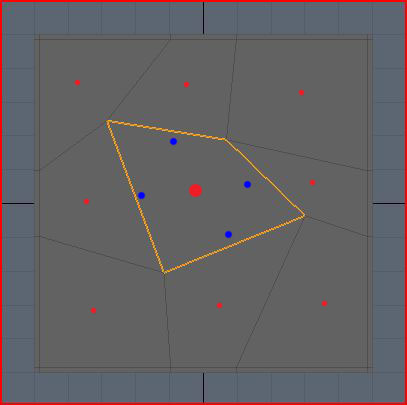
For the highlighted face only, I’ve drawn all the roughly where each new edge-point will go in blue:
Step Three
This step is a little bit more complicated, but very interesting. We’re going to see how we place the vertex-points from the original control points, and why they get placed there. This time, we use a weighted average to determine where the vertex-point will be placed. A weighted average is just a normal average, except you allow some values to have greater influence on the final result than others.
Before I begin with the details of this step, I need to define a term that you may have heard used in regards to subdivision surfaces – valence. The valence of a point is simply the number of edges that connect to that point. In the example mesh, you can see that all of the control points have a valence of 4.
Alright, I’m going to dive into some math here, but I’m also going to explain what the math actually means in real terms, so don’t be put off!
The new vertex-point is placed at:
(Q/n) + (2R/n) + (S(n-3)/n)
where n is the valence, Q is the average of the surrounding face points, R is the average of all surround edge midpoints, and S is the control point.
When you break this down, it’s actually fairly simple. Looking at our example, our control-points have a valence of 4, which means n = 4. Applying this to the formula, we now get:
(Q/4) + (R/2) + (S/4)
Much simpler! What does this mean though? Well, it says that a quarter of the weighting for the vertex-point comes from the average of surrounding face-points, half of it comes from the surrounding edge midpoints, and the last quarter comes from the original control-point.
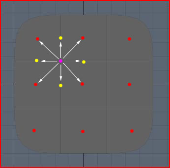
If we look at the top left control point in the highlighted face, Q is the average of the surrounding face-points, the red dots:

R is the average of the surrounding edge midpoints, the yellow dots. Note that the yellow dots represent the middle of the edge (just the average of the two end points) which is a little bit different from the edge-points we inserted above because they don’t factor in the nearby face-points.
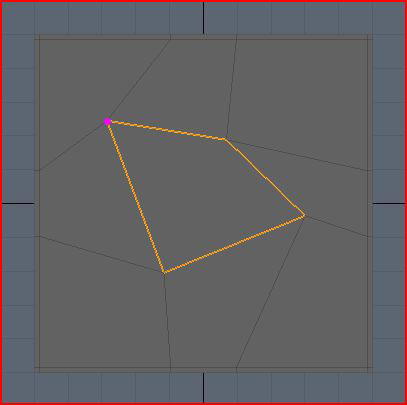
S is just the original control-point, the pink dot:
Below is my rough approximation of where all these averages come out, using the same color scheme as before. So the yellow dot is the average of all the yellow dots above, and the red dot is the average of all the red dots above.

Now all we do is take the weighted average of these points. So remember that the red dot accounts for a quarter, the yellow dot accounts for half, and the pink dot accounts for the final quarter. So the final resting place for the vertex-point should be somewhere near the yellow dot, slightly toward the pink dot, roughly where the pink dot is below:

So now I hope you can see why the control point is going to get pulled down and to the right. All the surrounding points just get averaged together and weighted to pull the vertex around. This means that if a control-point is next to a huge face, and three small faces, the huge face is going to pull that vertex towards it much more that the small faces do.
One other thing you can see from this is that if the mesh is split into regular faces, then the control point won’t move at all because the average of all the points will be the same as the original control point. The pull from each face-point and edge midpoint gets canceled out by a matching point on the other side:
Step Four
The final step is just to connect all the points. Confusingly, Modo has two ways to subdivide a mesh which actually return slightly different results. I don’t know why this is, or how the subdivision schemes differ, but they are close enough for all intents and purposes to call the same. For clarity, I’m using a screenshot from Modo where I have subdivided using the SDS subdivide command. For the highlighted face only, I’ve drawn the new face-point in red, the new edge-points in blue, and the moved vertex-points in pink:

Below is an overlay of the original control mesh for reference. As expected, you can see that the top left control-point gets pulled to the right. The same process is applied to all faces, resulting in four times as many quads as we had previously.
One More Thing
If you look at the formula for moving the control-point to its new location, you can see that not only are the immediate neighbor points used, so are the all the rest of the points in the adjoining faces. How much any single one of these surrounding points affects the control-point isn’t very clear from the original formula. This information is actually really easy to find out just by substituting in the surrounding points into the original formula.
I’m making the assumption from hereon out that all of the surrounding faces are quads to make things easier on myself. Also, I’m not going to write down each step of the expansion here since it got pretty big, but at the end, I got the following weights:
Control-point weight = (4n-7) / 4n
Edge-neighbor weight = 3 / 2n^2
Face-neighbor weight = 1 / 4n^2
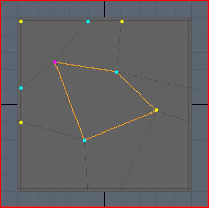
I’m using the term edge-neighbor to denote a neighboring point sharing the same edge as the control point, and face-neighbor as a neighbor that only shares the same face as the control-point. In the picture below, the edge-neighbors are cyan, and the face neighbors are yellow. Note that for quads, you have exactly n edge-neighbors, and n face-neighbors.
Applying this formula to various different valences, you get the following weights for a single point of the given type:
| Valence |
Control |
Edge Neighbor |
Face Neighbor |
| 3 | 5/12 | 3/18 | 1/36 |
| 4 | 9/16 | 3/32 | 1/64 |
| 5 | 13/20 | 3/50 | 1/100 |
| Infinity | 1 | 0 | 0 |
What does this mean? If we look at a the valence-4 row, you can see that if you move a face-neighbor, that’s going to affect the position of the vertex-point by 1/64th of however much you move it. So if you move it 64 cm on the x-axis, then the resulting vertex-point will move 1 cm in the same direction. I tested this scenario out in Modo, and it seems to match up very closely.
Clearly, the edge-neighbors are weighted more heavily than the face-neighbors, and the control-point itself always the most influence on the final vertex-point location. Remember though, each point represents a different thing (control-point, edge-neighbor, face-neighbor, nothing) depending on which particular face is getting subdivided!
It is interesting to note what happens as the valence gets larger and larger. The control-point influence tends towards 1, while all the neighboring points tend to zero. The reverse is also true, where at valence-4, the control-point weight is about 0.56, at valence-3 it is only 0.41 which means it is getting pulled around by its neighbors a lot more.
Wrap Up
I’ve learned a lot while investigating Catmull-Clark subdivision. There’s a lot more to learn, and a lot more to share, but I don’t have the time right now. This post was much longer than I thought it would be, so I’m going to look at some other aspects of subdivision modeling in later posts. One of the next things I’m going to look at will be how the rules change for boundary points, since these are often the bane of my modeling life…
I’m not really sure this will make me a better modeler, but at least I have a much better understanding of what will happen to my mesh when it gets subdivided. Hopefully I will be able to apply this knowledge to make my modeling process more predictable.
Remember that this only applies to non-boundary/crease points, and that different applications may use different weights for the points.
If you’re interested in checking out Modo, they have a 30 day trial available on the Luxology website. It’s really rather good, and I’ve seen some absolultely stunning images on the forums which were modeled and rendered using Modo.



Thanks a lot for the detailed explanation. I have been experimenting with the algorithm and cross-checking it with Lightwave 9.0 Catmull-Clark implementation. I have noticed discrepancies between LW9.0 implementation and the original work. Yet, I would like to ask about something else. How do you treat boundary edges? How do you calculate the new edge point of a boundary edge?
Thanks!
Hi,
So far I have found quite a lot of differences between how different packages treat boundary edges. Comparing, say, Modo and Max, I’ve noticed some significant differences in some situations. I can’t remember off-hand what the original paper said about these border cases – I’ll have to have another read.
Certainly, tools like vertex weight maps and edge creasing are completely inconsistent among the variety of pacakges which support Catmull-Clark surfaces – hence the reason why it’s often difficult to transport sub-d surfaces from one package to another. I’ve heard that Lightwave’s surfaces are particularly good, though I’m not sure how ‘good’ was measured.
I’ve been meaning to do some more research into subdivision surfaces in general now that DirectX 11 cards (with hardware tessellation units) are starting to make their way to the shops. I’ll let you know if I find something relevant.
Thank you so much for this great article. I have studied Catmull-Clark subdivision algorithm for quite a while and your article was at the top my list to read. Great work.
Regards,
Hamed
Hey Rory,
I’m a little late to the punch here, but awesome post.
I
I love Modo, and edge weighted sub-d, and I’m very much looking forward to OpenSubDiv and other implementations working their way into games.
I plan to make a very limited implementation of CC sub-d for Unity3d as a lodding system, and your post will really help me along that path.
Cheers,
Geoff
[…] http://www.rorydriscoll.com/2008/08/01/catmull-clark-subdivision-the-basics/ […]
I am reading RTR(real-time rendering),but it is a little bit difficulty for me to
catch up maybe since the illustration is so few.So i googled this article,i am lucky,because after reading this article,i understant how Catmull-Clark Subdivision works.thank you !!!!
Hi Rory,
How can i get the result:
Control-point weight = (4n-7) / 4n
Edge-neighbor weight = 3 / 2n^2
Face-neighbor weight = 1 / 4n^2
i can’t derive it.
the origin formula:
(Q/n) + (2R/n) + (S(n-3)/n)
I use E to stand for Edge-neighbor,F for Face-neighbor
then ,i get R=(Q+E+2S)/4,S=(Q+2E+(n-3)F)/n
I substitude E,F into the origin formula,but i can’t get the right weight.
Control-point weight = (4n-7) / 4n
Edge-neighbor weight = 3 / 2n^2
Face-neighbor weight = 1 / 4n^2
could you please clarify this for me? thx !
Thanks for this. Managed to get this implemented in my project (Bastard 3D) in under 30 minutes, well explained and to the point.
I’ve put the results on my facebook page (https://www.facebook.com/Bastard3d).
Please excuse the slightly weird name of the project, I’ll name it something sensible when I’m a bit further along with it 🙂
Thanks Again.
Chris Hebert