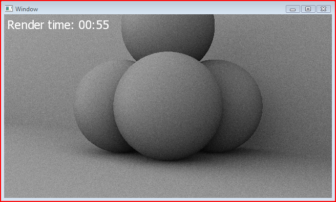
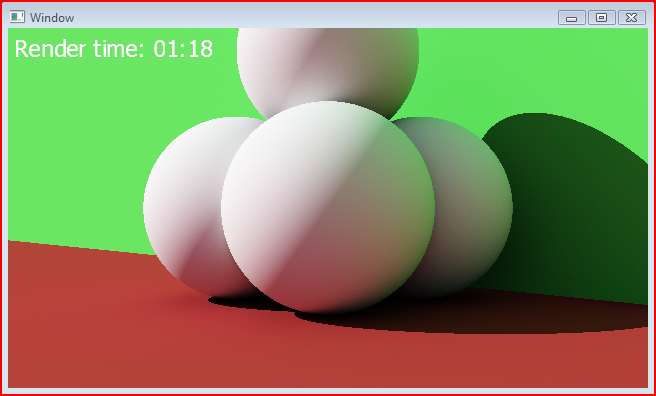
A couple of days ago, I compared the images my ambient occlusion integrator produced with those of Modo using similar settings. I noticed immediately how much ‘cleaner’ the render from Modo was. Clearly there was an issue with the way I was picking my samples, so I set about improving things.
My approach for generating the ambient occlusion rays was to generate uniform random samples over the hemisphere about the normal. Based on two random numbers in the range [0,1), I calculate the normalized sample direction using the following function:
Vector3 Sample::UniformSampleHemisphere(float u1, float u2)
{
	const float r = Sqrt(1.0f - u1 * u1);
	const float phi = 2 * kPi * u2;

	return Vector3(Cos(phi) * r, Sin(phi) * r, u1);
}
This generates points on a hemisphere from uniform variables u1 and u2, where each point has equal probability of being selected. The following image was generated with 256 random uniform samples:

It looks pretty noisy, that’s for sure. Part of the trouble comes from the fact that there’s no way to ensure that there’s an even distribution of the rays. A common way to alleviate this problem is to do stratified sampling instead of fully random sampling. The idea of stratified sampling is to split up the domain into evenly sized segments, and then to pick a random point from within each of those segments. You still get some randomness, but the points are more evenly distributed, which in turn reduces the variance. Less variance means less noise. Here’s the scene again, using 256 rays, but this time using stratified sampling:

As expected, it’s much less noisy, and for the same amount of computation!
Sampling for Diffuse Monte Carlo Estimator
The stratified sampler helps out with the indirect diffuse lighting calculation too, but one other thing you can do to reduce noise for the Monte Carlo estimator is to choose random values that have a similar ‘shape’ to the integral you are estimating. Looking at the integral for diffuse reflections, you will see the familiar cosine term inside the integral:
Where c is the diffuse material color, Li is the incoming radiance, and pi is the energy conservation constant.
Rather than wasting samples on areas of the integral where they will get mulitiplied out by the cosine term, why not just choose proportionally fewer samples in those areas?
Recall that the Monte Carlo estimator for an the integral of the function f(x), with probability density function p(x) is:
The probability density function is just a function that returns the probability that a particular value will be chosen. For the uniform hemisphere sampling function above, the pdf is just a constant, (1 / (2 * pi)). This makes the Monte Carlo estimator for the diffuse integral:
Rather than mutliply by the cosine term above, we just want to generate proportionally fewer rays at the bottom of the hemisphere. The integral of the pdf over the hemisphere must equal one, so by switching to a cosine-weighted sample distribution, the pdf becomes (cos(theta) / pi).
This makes the estimator:
Which cleans up rather nicely to:
Normally I would post a couple of images up for comparison’s sake, but in this case, the difference is pretty difficult to perceive without being able to compare one on top of the other. The difference is small, but it is definitely worth it!
The common way to generate a cosine weighted hemisphere sampler is to generate uniform points on a disk, and then project them up to the hemisphere. Here’s some code:
Vector3 Sample::CosineSampleHemisphere(float u1, float u2)
{
	const float r = Sqrt(u1);
	const float theta = 2 * kPi * u2;

	const float x = r * Cos(theta);
	const float y = r * Sin(theta);

	return Vector3(x, y, Sqrt(Max(0.0f, 1 - u1)));
}
Just by doing these two small steps, I’ve been able to clean up my images significantly. Here’s the scene from above again, this time with single bounce final gather with 256 rays, stratified cosine-sampled:

Next on my list is to take a look at path tracing, followed by irradiance caching (wasn’t that the point of all this?). This should allow me to get fairly cheap multi-bounce diffuse lighting.
Hi,
Nice article 🙂
I just have a question about the randomly generated point on the hemisphere.
In your code, you never use the normal to generate it. How do you know that the hemisphere is centered on the normal ?
This function just generates the ray direction in tangent space. It assumes that you will rotate the direction into world space afterwards.
I just use the normal and tangent vectors from the mesh (generating the bitangent from the cross product) and generate a basis (3×3 matrix) which transforms the ray from tangent space into world space.
You should change:
return Vector3(x, y, Sqrt(Max(0.0f, 1 – x * x – y * y)));
to
return Vector3(x, y, Sqrt(Max(0.0f, 1 – u1)));
because (x * x – y * y) = u1 in your example
to
return Vector3(x, y, Sqrt(1.0f – u1));
actualy
[…] same topic is discussed here: http://www.rorydriscoll.com/2009/01/07/better-sampling/ This entry was posted in Uncategorized. Bookmark the permalink. ← A simple […]
ShinZo, I’m pretty sure (x * x – y * y) is not u1, it’s u1*cos(2*theta), or 2*x*x-u1 (which is just as costly as the original formula).
Hmm, maybe I’m wrong… bah, I’m too tired to work it out.
Agree with Boris and others. it should be
return Vector3(x, y, Sqrt(1.0f – u1))
since 1-(r*cos(t))^2-(r*sin(t))^2 =>
1 – r^2 =>
1-u1
To make it a bit more explicit:
1 – x * x – y * y
1 – (r*cos(t))^2 – (r*sin(t))^2
1 – r^2*cos^2(t) – r^2*sin^2(t)
1 – r^2*(cos^2(t) + sin^2(t)) // Took out -r^2 as a factor
1 – (r^2*(1)) // Trig identities!
1 – r^2
1 – u1
Yay!
Ok, ok! Thanks for the clear explanation. I changed the post.
Hi Rory, I am still a bit confused by the transformation for the ray from tangent space into world space. Does it mean that I generate a normal vector using cosineSample(), and get the normal direction for a point from the mesh, then cross product them to obtain bitangent, finally get the transformation matrix? and multiply the matrix with the normal in tangent space then I can have the normal vector in world space, is this correct?
[…] we will use cosine-weighted sampling. More information on cosine-weighted sampling can be found here. Below u_1 and u_2 are uniform random variables. Ultimately, we will reorient the resultant vector […]
[…] little better. Let’s try 25 samples, evenly distributed around the hemisphere (incidentally see here for information on how to choose uniform sampling points on a hemisphere, using cosine weighting). […]